The pipe-network solver that shows its working.
Steady-state flows, pressures and temperatures for liquids, gases and heat, solved with named methods, stated assumptions and conservation residuals on every run. The results are verified against an independent reference problem set, so you can check the maths, not just trust it.
It runs in your browser, on any device, with nothing to install, and exports professional, print-ready reports of your results. Used by mechanical and process engineers, from A$20 a month rather than a five-figure desktop licence.
No account needed - try it on your own pipe.
Verified across liquid, gas, heat and non-Newtonian flow, EPANET-cross-checked on water. See the cases
Sign in free to save, share and reopen your work.
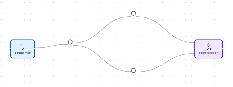
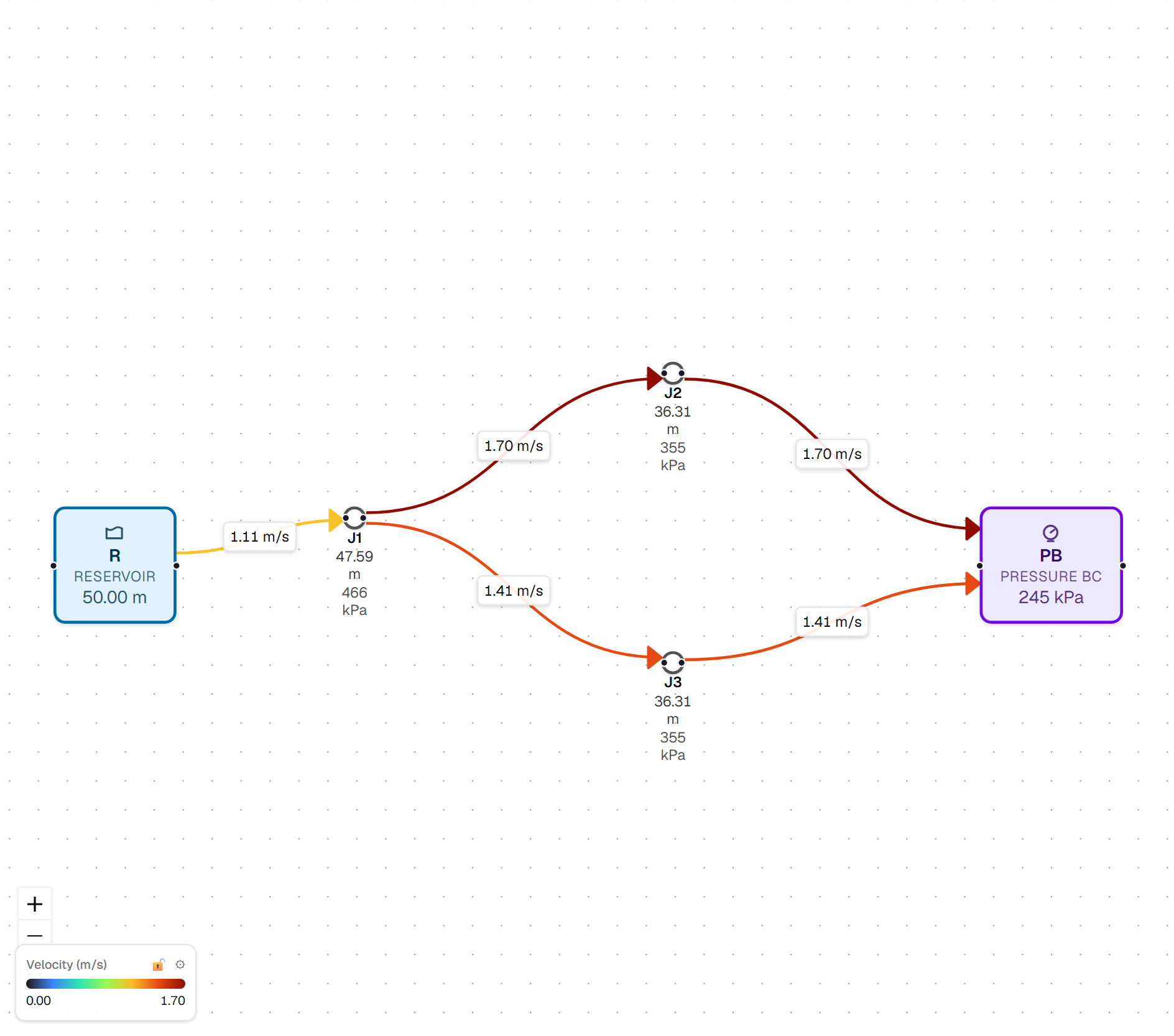
A looped pipe network, drawn and solved in your browser - one of 14 built-in, free-to-run examples.
Everything you need - for a fraction of the price.
Professional steady-state network analysis - liquids, gases and heat transfer - without the desktop licence, the install, or the five-figure price tag. From A$20 per month.
We listened to your frustrations
The reasons engineers told us they put off doing the calculation - and what we did about each one.
Is professional hydraulic software too expensive?
“The software is so expensive, and I barely use most of the features.”
A focused tool that does the steady-state analysis you actually reach for - from A$20 a month, not a five-figure desktop licence.
How quickly can I run a simple pipe-flow calculation?
“Sometimes I just want a simple calculation, and that takes too long in most packages.”
Open a browser tab, drop in a few pipes and a pump, and solve in seconds - no project setup, no ceremony.
Can I get to my pipe-network projects when I am on site?
“I do not have easy access to my projects, especially when I go to site.”
It runs in any browser, on any device. Sign in and your saved networks are right there - desk, site or home.
How long does Fluid Network Studio take to learn?
“The packages take too long to learn.”
If you can sketch a network, you can solve one. No manual and no training course - the tools are where you expect them.
Capabilities
A focused, auditable steady-state solver - four solve modes (liquid, liquid + heat, gas, gas + heat) wrapped in a fast schematic editor. The physics is verified against an independent reference problem set, and conservation residuals are reported on every solve.
A solver you can check, not just trust
Get steady-state flows and pressures across any network, however branched or looped, with the evidence they are right. Global-gradient (Todini–Pilati) solve with Darcy–Weisbach friction (Churchill), including non-Newtonian power-law and Bingham (homogeneous) fluids. Every result ships with machine-precision mass and energy residuals, so conservation is checked on every solve, not assumed. See the verification cases.
Catch heat loss before it costs you
Add heat to the model and see exactly where each pipe loses or gains it. Per-pipe heat loss or gain from inner films (Gnielinski or Dittus–Boelter), pipe walls and insulation, or a direct U value or imposed flux. Streams mix by enthalpy at junctions, and an energy balance runs on every solve.
Size gas lines with the same rigour as water
Model compressed air and process gases, not just liquids. Switch the fluid to a gas and solve in absolute pressure with mass-flow balances - isothermal, or with heat transfer by a temperature-and-density marching model. Air, methane, nitrogen and CO₂ presets plus custom gases, with optional Sutherland temperature-dependent viscosity and Peng–Robinson real-gas density.
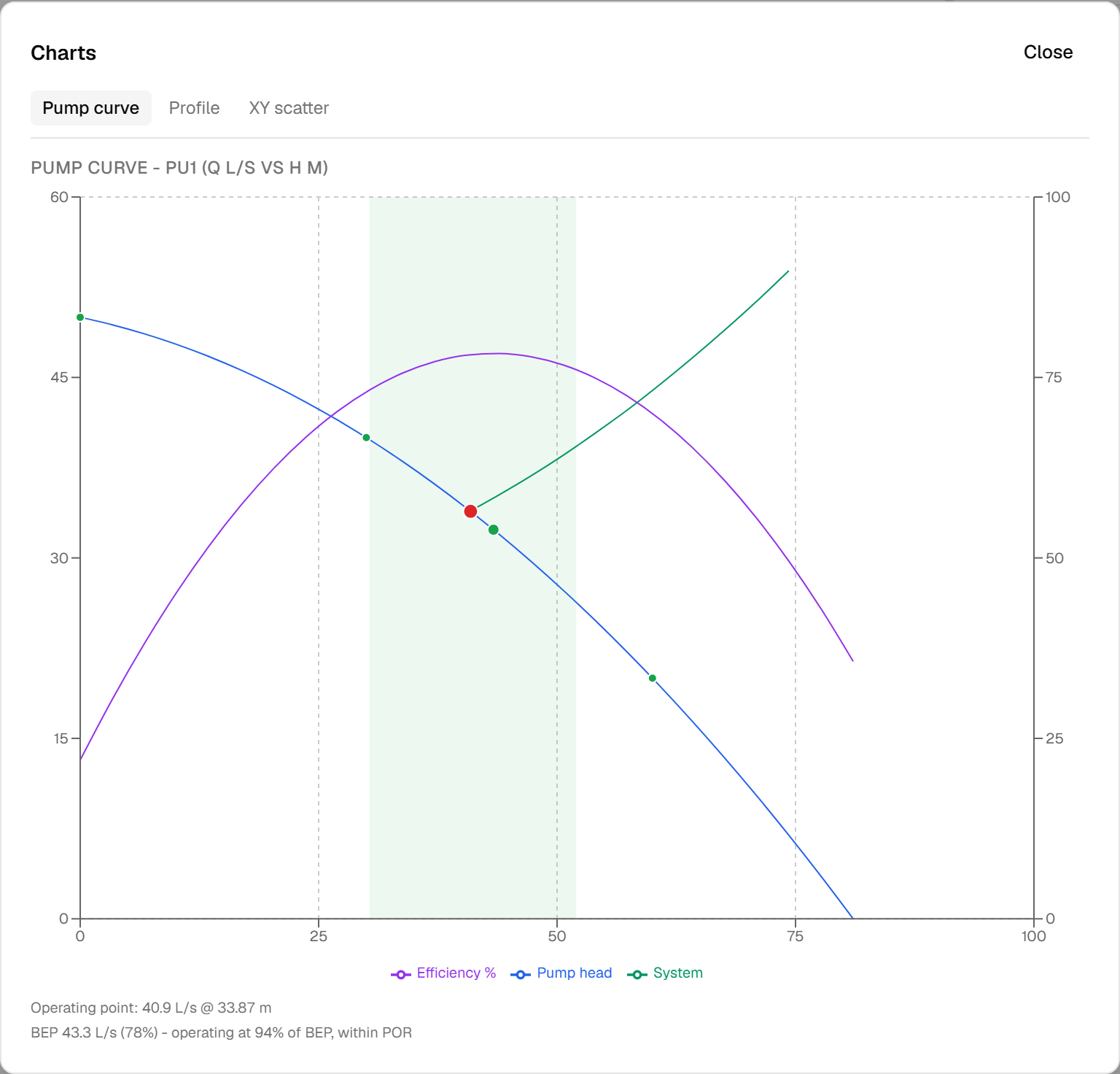
Know a pump will hit its duty point
Add rotating equipment and read off its operating point and power before you specify it. Pump curves with variable-speed affinity laws and operating-point charts; hydraulic and shaft power from a fixed efficiency or an efficiency curve with its best-efficiency point and operating-region check; NPSHa with a cavitation-risk flag. Fan Δp–Q curves scaled to inlet density; set-point compressors reporting discharge temperature and shaft power.
Model the whole system, and switch parts in and out
Tell the network what happens at its edges and junctions. Reservoirs, pressure and flow boundaries; node types (tee, elbow, cross) that carry their minor-loss K; standard fittings (Crane TP-410); and any connecting node can be closed to switch a whole branch off.
Work in the units you already use
Size pipes and switch units the way an engineer expects, with no conversion sheet. DN / Schedule pipe sizing (ASME B36.10M), material roughness presets, and switchable SI or imperial units (L/s, kPa, mm, m/s or gpm, psi, in, ft, ft/s).
Find velocity and pressure problems before commissioning
See the answer as colour, charts and tables, so problems stand out before they reach site. Colour the network by velocity, pressure or temperature; trace HGL and temperature profiles along any pipe run; per-component results with film, march and non-Newtonian flow-regime diagnostics; full tables with CSV export and a print-ready calculation report.
Your work leaves with you
Work entirely in the browser, save networks to a file, or sign in to store projects securely in the cloud, isolated to your account. Free local file save and EPANET .inp import mean your models are never trapped in the tool.
See the output
Real solver output from the built-in example networks - open any of them and reproduce it yourself.
Example networks
Worked examples across all four modes - water networks, hot-water mains losing heat, compressed air, fans, compressors and a hot gas line. Open any of them in the Studio and solve for free - no account needed.
Three-reservoir junction
The classic three-reservoir problem: three reservoirs at different water levels feed a common junction that also draws a fixed demand. The solver determines the magnitude and direction of flow in each pipe so that heads balance at the junction.
Open in Studio →Looped network
A single-loop network: a reservoir feeds a junction that splits into two parallel branches of different diameters, which recombine at a fixed-pressure boundary. The flow divides between the branches so that the head loss around the loop is consistent.
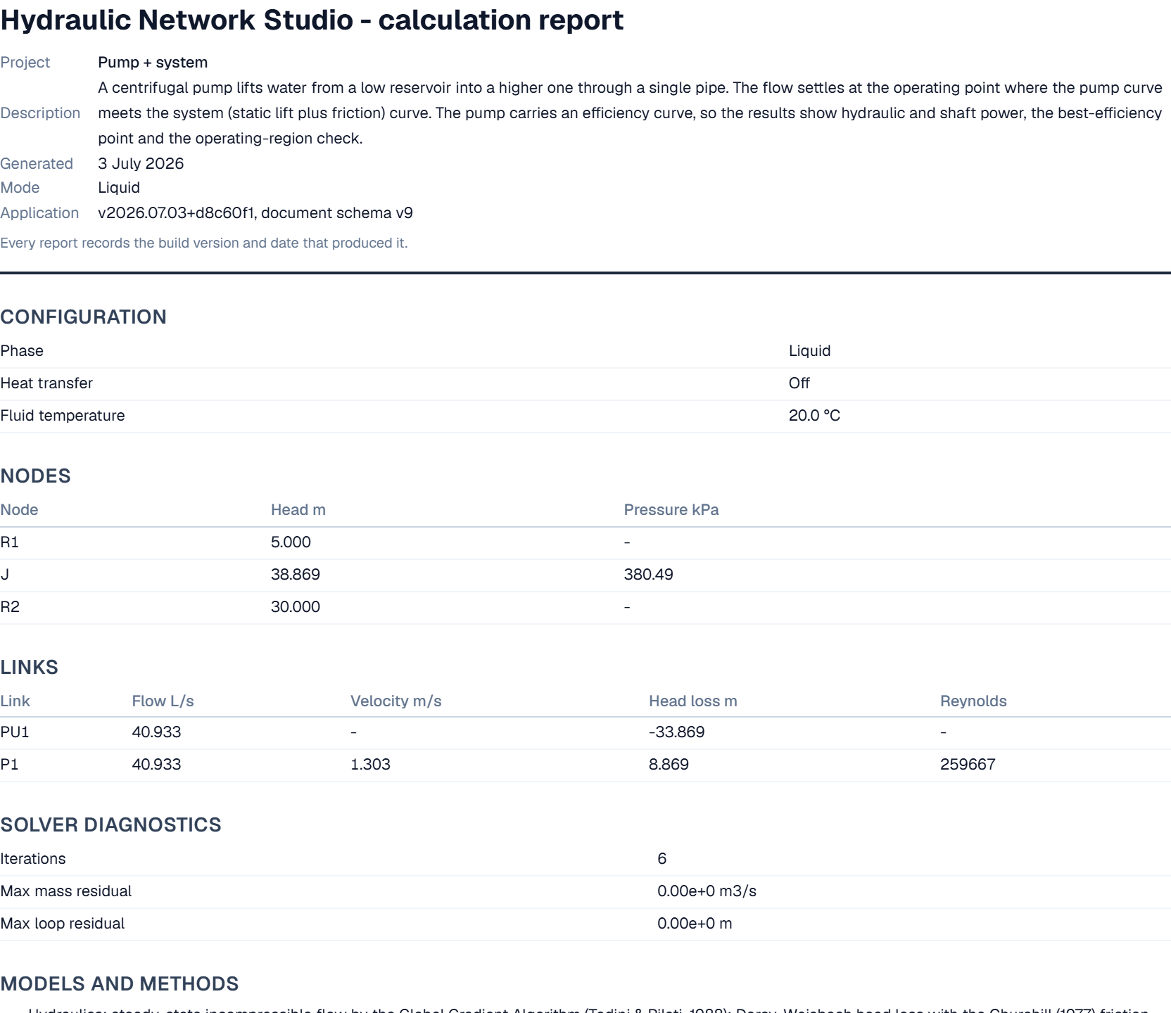
Open in Studio →Pump + system
A centrifugal pump lifts water from a low reservoir into a higher one through a single pipe. The flow settles at the operating point where the pump curve meets the system (static lift plus friction) curve. The pump carries an efficiency curve, so the results show hydraulic and shaft power, the best-efficiency point and the operating-region check.
Open in Studio →Supply line with fitting
A reservoir supplies a fixed demand through a single line containing an in-line 90° elbow. Demonstrates minor (fitting) losses alongside pipe friction, and how the gauge pressure at the outlet depends on elevation.
Open in Studio →Branched distribution
A branched distribution main supplies three demand points at different ground levels from a single reservoir. Demonstrates how pressure falls along the network with friction and varies from point to point with elevation.
Open in Studio →Hazen-Williams distribution
A water-distribution main sized with the Hazen-Williams method (the convention in water and fire engineering): a reservoir feeds a branched network of demand points, each pipe carrying its own C roughness coefficient. Switch the head-loss method in Configuration to compare against Darcy-Weisbach.
Open in Studio →Insulated hot-water main
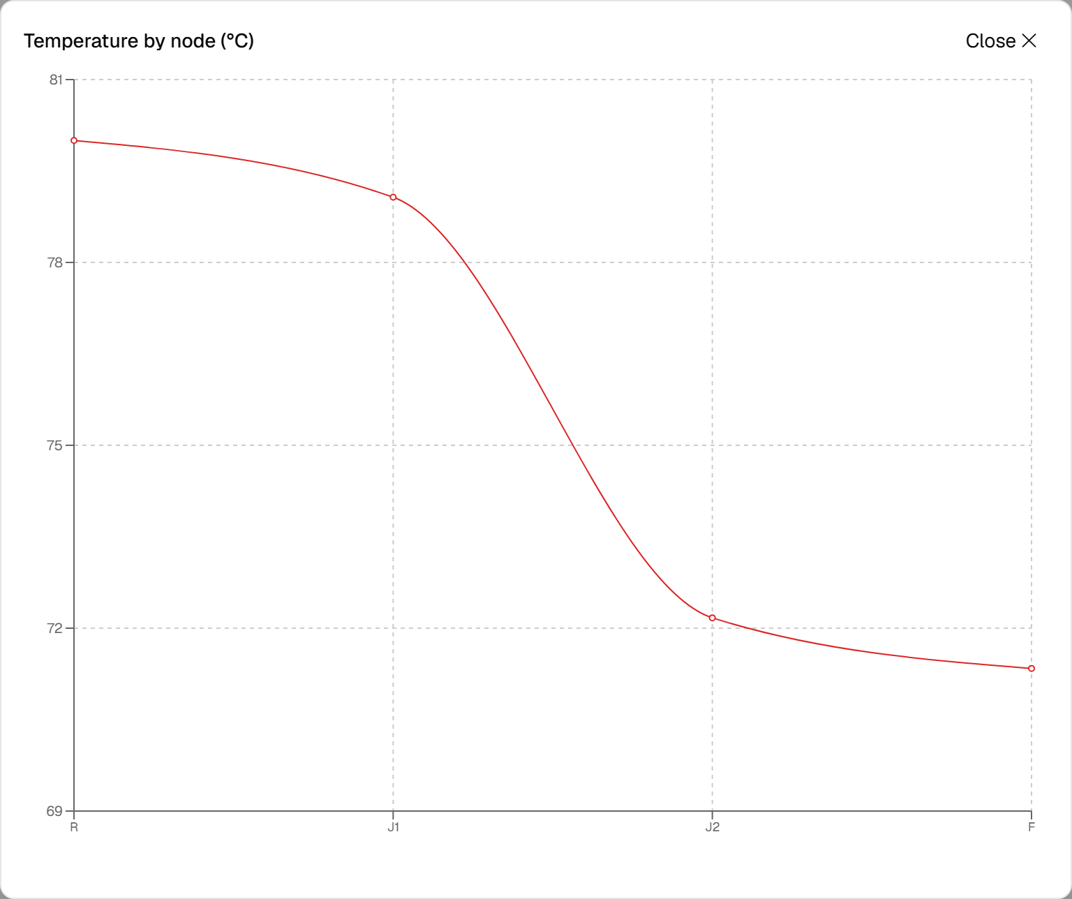
An 80 °C supply main in three 400 m segments: the first and last are insulated with 30 mm mineral wool, the middle one is bare. With heat transfer on, the solver builds each segment's heat loss from the Gnielinski film, the steel wall and the insulation - the bare segment loses far more temperature than both insulated segments together.
Open in Studio →Hot and cold mixing tee
A 70 °C stream (2 L/s) and a 15 °C stream (3 L/s) meet at a tee and mix by enthalpy to 37 °C. The combined flow then runs 300 m through a pipe losing heat to a 5 °C ambient (direct U), arriving just under 35 °C. Try Colour by → Temperature to see the mix.
Open in Studio →Compressed-air line
An air line at ~6 bar gauge feeding a 1.15 kg/s draw-off through two pipes of different diameter. With the gas phase selected, the solver works in absolute pressure with mass-flow balances - watch the velocity rise as the duct narrows and the density falls.
Open in Studio →Fan + duct (air)
A fan draws air from atmosphere and pushes it through a 60 m duct back to atmosphere. With the gas phase selected, the operating point settles where the fan's pressure-rise curve meets the duct's resistance - select the fan to see the Δp–Q chart and the operating-point marker.
Open in Studio →Compressor + line (air)
A compressor takes air at 200 kPa and compresses it to a 2:1 ratio (400 kPa), then a 150 m line carries it to a 300 kPa delivery point. Select the compressor to see the discharge temperature and shaft power; the network solves isothermally and the compressor reports T₂.
Open in Studio →Air blow-down (high velocity)
A short 20 m line discharging 300 kPa air to 120 kPa. The gas accelerates to about 210 m/s near the outlet - well past the compressibility-limit threshold - so the solver raises a high-velocity advisory. The isothermal model still solves, but the line is near its compressible capacity.
Open in Studio →Hot air line (cooling)
0.18 kg/s of 127 °C air enters a bare 300 m line at 500 kPa absolute and cools to a 15 °C ambient, arriving near ambient temperature. With heat transfer on, gas pipes solve by a segment march: watch the density RISE and the velocity FALL along the pipe as the gas cools - the opposite of an isothermal line. Try Colour by → Temperature.
Open in Studio →Power-law fluid network
A shear-thinning power-law fluid (consistency K = 0.5, behaviour index n = 0.5) fed from three reservoirs at 40, 28 and 15 m into a common junction. Select a pipe to see its flow regime and the Metzner-Reed generalised Reynolds number. Homogeneous, non-settling fluids only - turbulent friction uses smooth-pipe correlations.
Open in Studio →Bingham sludge line
A Bingham-plastic fluid (yield stress 8 Pa, plastic viscosity 0.03 Pa·s) pumped from a 30 m reservoir through a 100 m line to a draw-off. Select the pipe to see the laminar/turbulent regime via the Hanks transition. Homogeneous, non-settling fluids only - no settling-slurry or deposition behaviour is modelled.
Open in Studio →Tank fill with pump start/stop (transient)
A time-domain (transient) example: a pump lifts water into an open tank while a leak line drains it to a sink. The pump starts when the tank level falls below 2 m and stops when it rises above 5 m, so the level cycles within the deadband. Solve, then play or scrub the timeline; select the tank for its level-vs-time plot.
Open in Studio →Your data, your account
Straightforward about how your work and your details are handled - no lock-in, private by default, and honest about what is free and what needs a paid plan.
No lock-in
Your model stays yours. Save networks to a file and reopen them any time for free, and import an existing EPANET .inp model at no cost. Paid plans add export to CSV, Excel, EPANET .inp, PNG and SVG. So your models leave with you - whatever happens to the product, your files open in other tools.
Private by default
Saved projects are visible only to you. When you sign in and save to the cloud, each project is tied to your account - no other user can see it or open it. Your saved projects are stored in Australia (Sydney).
Payments handled by Stripe
If you subscribe, your card details are entered directly with Stripe and are never stored by Fluid Network Studio.
Australian owned and developed
Built and maintained in Australia (ABN 61 267 830 638), for engineers who want a straightforward, dependable tool.
More detail is in our Privacy Statement.
Pricing
Building and solving your own liquid networks is free; an account (also free) saves your work.
Explorer
Free
For: trying the tool and small networks. No account needed to solve.
- ✓Solve your own liquid (hydraulic) networks - no account needed
- ✓Up to 20 elements without an account, 40 once you sign in
- ✓Run the built-in example networks
- ✓All editor and visualisation tools
- ✓Sign in free to save to a local file
Basic
14-day free trial
For: individual engineers doing everyday liquid work - pump duty, HVAC hydronics, cooling water.
- ✓Everything in Explorer
- ✓Up to 1,000 elements per network
- ✓Cloud save & load (up to 100 projects)
- ✓Export results (CSV and calculation report)
Advanced
14-day free trial
For: process engineers who need gas, heat or non-Newtonian flow.
- ✓Everything in Basic
- ✓Compressible gas networks, with compressors and fans
- ✓Non-Newtonian fluids (power-law and Bingham)
- ✓Heat transfer - per-pipe loss or gain, mixing and energy balance
Team
Contact us
For: offices that share models and want volume licensing.
- ✓Everything in Advanced
- ✓Shared projects
- ✓Priority support
- ✓Volume licensing
Volume licensing for teams and offices.
Cloud save, sharing and export (CSV, Excel, EPANET .inp, PNG, SVG) are on the paid plans.
When do I need Advanced?
Basic covers most liquid work: water distribution, pump sizing, HVAC hydronics, cooling-water loops.
Choose Advanced for: compressed air and gas lines, hot lines losing heat, homogeneous slurries and pastes (power-law and Bingham), and thermal networks.
Important - please read
Fluid Network Studio is provided for general information and preliminary analysis only. Results depend entirely on the data you enter and on modelling assumptions, and they are not a substitute for the judgement of a qualified engineer. You are responsible for independently checking any result before relying on it. The tool is provided “as is”, without warranty of any kind, and your use of it is subject to the Terms of Use & Disclaimer and the Privacy Statement.