How Fluid Network Studio works
Published . Last updated .
Fluid Network Studio takes a pipe network from a sketch to a solved, conserved result in four steps: draw it, choose the fluid and solve mode, solve, and read the results. The physics runs entirely in your browser - there is no solve server - and every result ships with its conservation residuals so you can see the maths balanced. Here is the whole workflow.
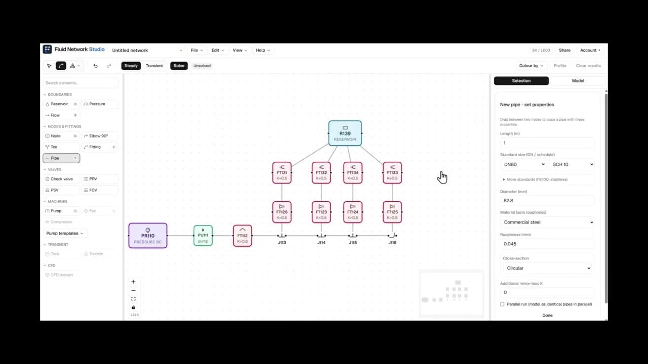 Play the demo (1:56)
1. Draw the network on the canvas
You build the network as a schematic on the canvas, the way you would sketch it on paper. The building blocks are:
- Reservoirs - a fixed head (a tank, a mains connection, an open atmosphere).
- Boundaries - demand or flow boundaries (a fixed draw-off or injection, in L/s or kg/s) and pressure boundaries (a fixed pressure or gauge pressure).
- Junctions and nodes - the connection points. Node types such as elbow, tee and cross prefill their own minor-loss K, and any connecting node can be closed to switch a whole branch off.
- Pipes - with length, diameter (including DN and Schedule sizing) and a material roughness, carrying optional thermal properties when heat transfer is on.
- Pumps - with a head-flow curve and an optional efficiency curve, and variable speed via the affinity laws.
- Fans and compressors - for gas networks: a fan with a pressure-rise curve, or a set-point compressor.
- Fittings and loss elements - a fixed-K minor-loss library (50 fittings): 44 carry coefficients of the class published in Crane TP-410, three are ASHRAE duct values and three are manufacturer-typical figures. Every K is a prefill you can edit. Plus orifice plates, sudden expansions and contractions, and non-circular (rectangular and oval) ducts sized by hydraulic diameter.
- Control valves - non-return check valves that stop reverse flow, and PRV, PSV and FCV control valves that hold a pressure or flow set-point (steady-state control law).
You add elements from the palette, connect them, and edit each one's properties in the inspector. You can load any of the 20 built-in examples as a starting point.
If you would rather describe the system than draw it, build it with AI: you give the AI assistant you already use a guide the Studio publishes, describe the system in plain English, and paste the reply back. Every unit, connection and library name is checked before anything reaches the canvas, and you then solve and edit it like any other network.
2. Choose the fluid and the solve mode
Pick the working fluid and the mode that matches the problem. There are four solve modes:
- Incompressible liquid - water and process liquids at constant density, solved in head. This is the default and is available on every plan, including free.
- Liquid with heat transfer - the same network with per-pipe heat loss or gain and enthalpy mixing at junctions. Advanced plan.
- Compressible gas (isothermal) - air and process gases, solved in absolute pressure with mass-flow balances and varying density. Advanced plan.
- Gas with a thermal march - a compressible gas line that also exchanges heat, solved with a temperature-and-density march along each pipe. Advanced plan.
The fluid library has 25 liquid presets (water with temperature-dependent properties among them), 12 gas presets (air, methane, nitrogen, carbon dioxide, oxygen, hydrogen and more) and custom fluids, plus homogeneous non-Newtonian rheology (power-law and Bingham plastic), which also needs the Advanced plan. Incompressible water analysis on the free plan covers the great majority of everyday pipe-flow work. Gas, heat transfer and non-Newtonian fluids are the Advanced additions.
Steady, or over time. Each network solves at steady state, or in transient (extended-period) mode: give a reservoir tank storage, put valves on schedules or level triggers, let pumps start and stop with hysteresis, vary demands through the day, then play or scrub the timeline and plot any element over time. The engine is quasi-steady - it re-solves the verified steady network at each timestep and integrates tank levels - so water hammer and surge remain out of scope. Transient mode runs on incompressible-liquid networks and is available on every plan, including free.
3. Solve
Press Solve. Fluid Network Studio assembles the network with the Global Gradient Algorithm (Todini and Pilati, 1988) - the incidence-matrix formulation behind EPANET - and converges it with Newton iterations. Friction head loss is Darcy-Weisbach with the Churchill friction factor. Fittings add fixed-K minor losses, pump curves are least-squares fits, and variable-speed machines use the affinity laws.
In the other modes the same core is reused. Heat transfer adds inner-film coefficients (Gnielinski or Dittus-Boelter) through a composite wall and insulation resistance with an outer film. The gas modes solve in pressure-squared with the isothermal pipe relation, and the gas thermal march integrates friction, acceleration and wall heat along each segment with Sutherland temperature-dependent viscosity. Whatever the mode, an energy and mass balance runs on every solve and the residuals are reported - conservation is checked, not assumed. The results are verified against a published reference problem set spanning liquid, gas, heat and non-Newtonian flow, with OWA-EPANET 2.2 as the independent incompressible-water cross-check and NASA's GFSSP as the independent-code reference for the network and component cases. The named methods are set out in the glossary, and the primary sources are listed in the references below.
4. Read the results
The answer comes back as colour, charts, tables and numbers:
- Per-element results - flow, velocity, head, pressure and (in heat modes) temperature on every pipe and node, plus film, march and non-Newtonian flow-regime diagnostics where they apply.
- Colour-coding - shade the network by velocity, pressure or temperature to see where the action is at a glance.
- Profiles - trace the hydraulic grade line or the temperature along any pipe run.
- Time plots - in transient mode, plot any element over time and export the time series to CSV.
- Pump and fan charts - the curve, the operating point, the best-efficiency point and the operating-region check, plus NPSHa with a cavitation-risk flag.
- Validation panel and advisories - design advisories such as high velocity or negative pressure, with click-to-locate, against limits you can configure.
- Tables, CSV and a calculation report - full result tables, CSV export, and a print-ready calculation report. Every report records the build version and date that produced it.
5. Save to the cloud or export
Work entirely in the browser if you like, save a network to a JSON file on your machine, or sign in to store projects securely in the cloud, isolated to your account. Export results to CSV or generate the calculation report when you need a record.
Reproducible results
The solver is deterministic: the same inputs, solved on the same build, produce the same result every time. Every calculation report records the build version and the date it was produced, alongside the document schema version, so a result you file today can be reproduced and audited later.
References
Every method above is a published one, and none of it is ours. These are the primary sources, so you can check the physics rather than take our word for it.
Network solution
- Todini, E. and Pilati, S. (1988), "A gradient algorithm for the analysis of pipe networks", in Computer Applications in Water Supply, Volume 1: Systems Analysis and Simulation, John Wiley and Sons. The Global Gradient Algorithm. Its use in EPANET is described in the EPANET analysis algorithms documentation.
- Rossman, L. A. (2000), EPANET 2 Users Manual, US Environmental Protection Agency. epa.gov/water-research/epanet
- OWA-EPANET 2.2, the Open Water Analytics build used as the incompressible-water cross-check. github.com/OpenWaterAnalytics/EPANET
- NASA/TP-2016-218218, Generalized Fluid System Simulation Program (GFSSP), the independent finite-volume code the network and component cases are cross-checked against. NASA NTRS
- Cross, H. (1936), Analysis of Flow in Networks of Conduits or Conductors, Bulletin No. 286, University of Illinois Engineering Experiment Station. The hand method the Global Gradient Algorithm replaced. IDEALS
Friction and minor losses
- Colebrook, C. F. (1939), "Turbulent flow in pipes, with particular reference to the transition region between the smooth and rough pipe laws", Journal of the Institution of Civil Engineers. doi.org/10.1680/ijoti.1939.13150
- Moody, L. F. (1944), "Friction factors for pipe flow", Transactions of the ASME. ASME Digital Collection
- Churchill, S. W. (1977), "Friction-factor equation spans all fluid-flow regimes", Chemical Engineering, Vol. 84, No. 24, pp. 91-92. The explicit correlation the solver evaluates.
- Crane Co., Technical Paper No. 410: Flow of Fluids Through Valves, Fittings and Pipe, the published source for the class of fixed-K coefficients the fitting library carries. tp410.com
What is checked, and what is not, in the minor-loss library. The fixed-K method is verified. The parameterised orifice, sudden-expansion and sudden-contraction elements are cross-checked against NASA GFSSP and the exact Borda-Carnot result, and the non-circular duct against a closed-form hydraulic-diameter calculation, all on the verification page. The individual K values in the fitting library are not. No published case compares a library K against TP-410: the tables are a copyrighted commercial publication we do not reproduce, and a case that compared the library against the figure it was taken from would only be checking our transcription, not the physics. So read the library as a well-sourced prefill rather than a verified value. Where the number matters, enter your own datasheet or measured K, or let the Studio convert a manufacturer's Kv or Cv, or a rated pressure drop at a rated flow, straight into one.
Heat transfer and non-Newtonian flow
- Gnielinski, V. (1976), "New equations for heat and mass transfer in turbulent pipe and channel flow", International Chemical Engineering, and Dittus, F. W. and Boelter, L. M. K. (1930), University of California Publications in Engineering, for the inner-film coefficients.
- Incropera, F. P. and DeWitt, D. P., Fundamentals of Heat and Mass Transfer, Wiley, for the composite-cylinder resistance network.
- Sutherland, W. (1893), "The viscosity of gases and molecular force", Philosophical Magazine, Series 5, for the temperature-dependent gas viscosity used in the thermal march.
- Metzner, A. B. and Reed, J. C. (1955), "Flow of non-Newtonian fluids: correlation of the laminar, transition and turbulent-flow regions", AIChE Journal. doi.org/10.1002/aic.690010409
- Dodge, D. W. and Metzner, A. B. (1959), "Turbulent flow of non-Newtonian systems", AIChE Journal. doi.org/10.1002/aic.690050214
See it on a real network
Reading about a solve is no substitute for running one. The built-in examples cover all four solve modes, steady and over time - water networks, an insulated hot-water main losing heat, a compressed-air line, a fan and duct, a compressor, a cooling hot-gas line, homogeneous non-Newtonian fluids, and a tank-and-pump system running over time. Open any of them and solve for free.
A good first run is the pump and system example (the operating point), the compressed-air line (a gas network) or the insulated hot-water main (heat loss along a line). For how the same physics meets a design task, see the application guides for compressed air system design, pipe heat loss and pump system design.
Fluid Network Studio is built to support engineering work, not to replace a qualified engineer's judgement - check every result in the context of your application before relying on it.
Launch the Studio - free to build and to run the 20 built-in examples.